Building Adam Optimization | Fernando Borrero Granell

Table of Contents:

Introduction.
Theory.
Results.
License.

1. Introduction

In this side project, I tackled the challenge of creating an implementation of the Adam optimizer completely from scratch, without relying on pre-existing machine learning libraries (this involved writing all the code myself). While many popular deep learning libraries offer sophisticated optimization algorithms like Adam, implementing them from scratch can provide a deeper understanding of their inner workings.

Adam (short for Adaptive Moment Estimation) is a widely used optimization algorithm for deep learning that combines the benefits of two other popular optimization methods, Adagrad and RMSprop. The main goal of Adam is to improve the efficiency and speed of gradient-based optimization algorithms.

You can check the code here.

2. Theory

This section will explain the inner workings of three optimization algorithms: Batch gradient descent, Mini-batch gradient descent, and Adam’s algorithm.

2.1 Mini-batch gradient descent.

Unlike batch gradient descent, which updates the parameters using the gradients computed on the entire training dataset, mini-batch gradient descent updates the parameters using a subset, or “mini-batch,” of the training data at each iteration. This approach can be more efficient and practical for training large datasets, as it allows the algorithm to make progress with fewer computations and reduces memory requirements.

In this project I chose a \(\text{mini-batch-size}=64\) (using a power of two is necessary for performance reasons.)

2.2 Weighted exponential averages.

A weighted exponential average is a statistical technique commonly used for calculating a smoothed average of a set of values by placing greater weight on recent observations while still considering past ones. The recursive formula is

\[V_t=\beta V_{t-1}+(1-\beta)\theta_t\]

If we apply the formula recursively, we obtain

\[V_t=\beta (\beta V_{t-2}+(1-\beta)\theta_{t-1})+(1-\beta)\theta_t = \beta^2V_{t-2}+\beta(1-\beta)\theta_{t-1}+(1-\beta)\theta_t =\] \[= \beta^2 (\beta V_{t-3}+(1-\beta)\theta_{t-2})+\beta(1-\beta)\theta_{t-1}+(1-\beta)\theta_t =\] \[\beta^3V_{t-3}+\beta^2(1-\beta)\theta_{t-2}+\beta(1-\beta)\theta_{t-1}+(1-\beta)\theta_t\]

We can see that the formula generalizes to the expression below:

\[V_t = \sum_{i=1}^t \beta^{t-i}(1-\beta) \theta_i\]

The value of \(V_t\) is a weighted average, where the weight of the measurement \(\theta_i\) decays exponentially as we get away from the current value \(t\), and that is why it’s called exponential weighted average. However this mean is not normalized for \(\theta\), and that is where the bias term correction comes into play:

\[V_{t,corrected} = \frac{V_t}{1-\beta^t}\]

We have seen that this method assigns exponentially decreasing weights to the past observations, with the weights determined by a smoothing factor or decay rate that controls how quickly the weights decrease over time. The weighted exponential average can be useful for reducing the impact of noise or fluctuations in data while preserving important patterns or trends.

2.3 Adaptive Moment Estimation (Adam) algorithm.

Adam algorithm uses the power of weighted exponential averages twice. Instead of taking steps proportional to the current gradient, Adam uses the first moment (weighted exponential average of the gradients). Thanks to this, gradients in opposite directions (oscillations) will cancel each other out, and we’ll increase convergence. This technique then divides the first moment by the root square of the second moment (weighted exponential average of the squared gradients), with works as a normalizer.

We can compute everything by integrating this code in our update_parameters step of gradient descent.

On iteration t:
    # Computing the first moment.
    VdW = b1*VdW + (1-b1)*dW
    Vdb = b1*vdb + (1-b1)*dW
    
    # Computing the second moment.
    SdW = b2*SdW + (1-b2)*dW**2
    Sdb = b2*Sdb + (1-b2)*db**2

    # Correcting the moments with bias term.
    VdW_cor = VdW/(1-b1**t)
    Vdb_cor = Vdb/(1-b1**t)
    SdW_cor = SdW/(1-b2**t)
    Sdb_cor = Sdb/(1-b2**t)

    # Gradient descent step.
    W -= learning_rate*Vdw_cor/(np.sqrt(SdW_cor)+epsilon)
    b -= learning_rate*Vdb_cor/(np.sqrt(Sdb_cor)+epsilon)

2.3 Learning rate decay.

If we’re working with mini-batch, we will have some noise in each iteration. Nevertheless, the average direction is the same as the gradient, and at the end we will oscillate around the minimum. We can solve this final oscilation by slowly reducing the learning rate. In this case, I have chosen to work with the following decay:

\[\alpha = \frac{1}{1+\text{decayRate}\times \text{epochNumber}}\alpha_0\]

Instead of decaying the learning rate in each epoch, it’s possible to reduce it after certain intervals. I chose to work with a decay_interval of 5, which means the rate decays every 5 epochs.

3. Results

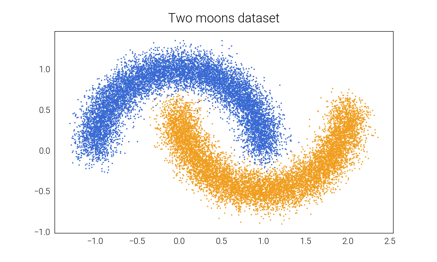
In this section, we will compare the performance of three different optimization algorithms for classifying a “two-moons” dataset.

Examining the training curves, it becomes evident that Adam’s algorithm is the most efficient, converging in just a few epochs. Mini-batch gradient descent follows closely behind, but is not as efficient. Finally, we have batch gradient descent, which is significantly less efficient and unable to reach a satisfactory solution within the same number of epochs.

The accuracy of the model is much higher for Adam and Mini-batch gradient descent, at around 99%, compared to batch gradient descent’s 86%. Although Adam and Mini-batch are both highly accurate, Adam emerges as the clear winner, achieving the most optimal solution five times faster.

In conclusion, the results of our comparison of optimization algorithms demonstrate the importance of carefully selecting the right method for the given problem. While batch gradient descent may be suitable for small datasets or problems with relatively simple optimization landscapes, Adam and mini-batch gradient descent are more efficient and better suited for larger datasets and more complex problems. Understanding the trade-offs and benefits of each optimization algorithm is essential for achieving optimal performance and training efficiency.

4. License

This project is intended for educational purposes only and all materials, including but not limited to code, data, and documentation, are available for free use, modification, and distribution.