Deep Learning with matrices
Personal implementation of a neural network trained for computer vision classification.

Table of Contents:
1. Introduction
Neural networks are widely regarded as one of the most powerful tools in the field of artificial intelligence. However, building such networks can be a daunting task, and that’s why people typically rely on third-party, sophisticated libraries like Tensorflow to reuse other people’s work and streamline the process.
In this particular side project, I took on the challenge of creating a neural network completely from scratch, without any assistance from machine learning libraries. This meant writing all the code myself and relying solely on numpy matrices. Thanks to all of this work, I was able to gain a deeper understanding of the fundamental workings of neural networks.
You can check the code here.
2. Theory
In this section, I will provide an explanation of the theoretical framework of this project. This will involve deriving the mathematical expressions that are used in creating neural networks.
In order to train the model, we need to evaluate its predictions on some data. To achieve this, we use a cost function. We’re working with a binary classification problem, thus we use the cross-entropy loss function.
\[L(a^{[L]},y) = -\left[ y \ln (a^{[L]}) + (1-y) \ln (1-a^{[L]})\right]\]where \(a^{[L]}\) is the activation value of the output layer. In order to define the neural network we need its parameters, which are stored in matrices \(W^{[l]}\) and vectors \(b^{[l]}\).
\[W^{[l]}= \begin{pmatrix} \leftarrow \vec{w}_1^{[l]} \rightarrow \\ \leftarrow \vec{w}_2^{[l]}\rightarrow \\ \vdots \\ \leftarrow \vec{w}_{n^{[l]}}^{[l]}\rightarrow \\ \end{pmatrix} \qquad b^{[l]}= \begin{pmatrix} b_1^{[l]} \\ b_2^{[l]} \\ \vdots \\ b_{n^{[l]}}^{[l]} \\ \end{pmatrix}\]We compute the activation values through forward propagation while using the former parameters.
\[\vec{a}^{[l]} = g^{[l]}(\vec{z}^{[l]}) = g^{[l]}(W^{[l]}\cdot \vec{a}^{[l-1]}+\vec{b}^{[l]})\]This expression can also be written for a specific unit \(u\) of the layer \(l\) as.
\[a^{[l]}_u = g^{[l]} \left( \sum_{j=1}^{n^{[l-1]}} w_{u,j}^{[l]} a_j^{[l-1]}+b_u^{[l]} \right)\]2.1 Layer L
The output layer is the easiest to solve since it works with one single neuron. If we apply a bit of calculus, we can compute the derivative of the loss function as
\[\frac{\partial L}{\partial a^{[L]}} = L'(a^{[L]}) = -\frac{y}{a^{[L]}}+\frac{1-y}{1-a^{[L]}}\]The output layer is working with a sigmoid activation function, thus \(a^{[L]}=g(z^{[L]})= \frac{1}{1+e^{-z^{[L]}}}\). We can compute its derivate by applying the chain rule from calculus
\[g'(z^{[L]})=\frac{(-1)(-1)e^{-z^{[L]}}}{(1+e^{-z^{[L]}})^2}=\frac{(1+e^{-z^{[L]}})-1}{(1+e^{-z^{[L]}})^2}= \frac{1}{1+e^{-z^{[L]}}}-\frac{1}{(1+e^{-z^{[L]}})^2}=a^{[L]}(1-a^{[L]})\]Now we are ready to easily compute the derivate from respect to \(z^{[L]}\) as follows
\[\frac{\partial L}{\partial z^{[L]}} = \frac{\partial L}{\partial a^{[L]}}\frac{\partial a^{[L]}}{\partial z^{[L]}} = \left( -\frac{y}{a^{[L]}}+\frac{1-y}{1-a^{[L]}} \right) a^{[L]}(1-a^{[L]})\] \[= -y(1-a^{[L]})+(1-y)a^{[L]}=-y+a^{[L]}y+a^{[L]}-a^{[L]}y=a^{[L]}-y\]The last gradient computed for the layer is those with respect to the parameters, which we will need to perform gradient descent.
\[\frac{\partial L}{\partial w^{[L]}_j} = \frac{\partial L}{\partial z^{[L]}} \frac{\partial z^{[L]}}{w^{[L]}_j} = \frac{\partial L}{\partial z^{[L]}} a_j ^{[L-1]} \Rightarrow \frac{\partial L}{\partial\vec{w}^{[L]}} \equiv \frac{\partial L}{\partial z^{[L]}} \vec{a} ^{[L-1]T}\] \[\frac{\partial L}{\partial b^{[L]}} = \frac{\partial L}{\partial z^{[L]}} \frac{\partial z^{[L]}}{b^{[L]}} = \frac{\partial L}{\partial z^{[L]}}\]2.2 Layer L-1
To keep derivating now we have to go back to the previous layer (where we have \(n^{[L-1]}\) units).
\[\frac{\partial L}{\partial a_u^{[L-1]}} = \frac{\partial L}{\partial z^{[L]}} \frac{\partial z^{[L]}}{\partial a_u^{[L-1]}} = \frac{\partial L}{\partial z^{[L]}} w^{[L]}_u \Rightarrow \frac{\partial L}{\partial \vec{a}^{[L-1]}} \equiv \frac{\partial L}{\partial z^{[L]}} \vec{w}^{[L]T}\]Now the derivate with respect to \(z\) is computed, where the hidden activation functions \(g\) are ReLUs.
\[\frac{\partial L}{\partial z_u^{[L-1]}} = \frac{\partial L}{\partial a_u^{[L-1]}} \frac{\partial a_u^{[L-1]}}{\partial z_u^{[L-1]}} = \frac{\partial L}{\partial a_u^{[L-1]}}g'(z_u^{[L-1]}) \Rightarrow \frac{\partial L}{\partial\vec{z}^{[L-1]}} \equiv \frac{\partial L}{\partial\vec{a}^{[L-1]}} * g'(\vec{z}^{[L-1]})\]As in the previous layer, the last step in this layer is to compute the gradients with respect to the parameters.
\[\frac{\partial L}{\partial w^{[L-1]}_{u,q}} = \frac{\partial L}{\partial z_u^{[L-1]}} \frac{\partial z_u^{[L-1]}}{\partial w^{[L-1]}_{u,q}} = \frac{\partial L}{\partial z_u^{[L-1]}} a_q^{[L-2]} \Rightarrow \frac{\partial L}{\partial W^{[L-1]}} = \frac{\partial L}{\partial\vec{z}^{[L-1]}} \vec{a}^{[L-2]T}\] \[\frac{\partial L}{\partial b^{[L-1]}_{u}} = \frac{\partial L}{\partial z_u^{[L-1]}} \frac{\partial z_u^{[L-1]}}{\partial b^{[L-1]}_{u}} = \frac{\partial L}{\partial z_u^{[L-1]}} 1\Rightarrow \frac{\partial L}{\partial\vec{b}^{[L-1]}} = \frac{\partial L}{\partial\vec{z}^{[L-1]}}\]2.3 Layer L-2.
This step is a bit more complex than the previous one \(L \rightarrow L-1\), since we go from one layer with \(n^{[L-1]}\) units to one with \(n^{[L-2]}\) neurons.
\[\frac{\partial L}{\partial a_u^{[L-2]}} = \sum_{p=1}^{n^{[L-1]}} \frac{\partial L}{\partial z_p^{[L-1]}} \frac{\partial z_p^{[L-1]}}{\partial a_u^{[L-2]}} = \sum_{p=1}^{n^{[L-1]}} \frac{\partial L}{\partial z_p^{[L-1]}} W_{p,u}^{[L-1]} \Rightarrow \frac{\partial L}{\partial\vec{a}^{[L-2]}} = W^{[L-1]T} \frac{\partial L}{\partial\vec{z}^{[L-1]}}\]With which we can easily compute the derivate with respect to the linear activation values.
\[\frac{\partial L}{\partial z_u^{[L-2]}} = \frac{\partial L}{\partial a_u^{[L-2]}} \frac{\partial a_u^{[L-2]}}{dz_u^{[L-2]}}= \frac{\partial L}{\partial a_u^{[L-2]}} g'(z_u^{[L-2]}) \Rightarrow \frac{\partial L}{\partial\vec{z}^{[L-2]}} = W^{[L-1]T} \frac{\partial L}{\partial\vec{z}^{[L-1]}}*g'(\vec{z}^{[L-2]})\]Now we could compute the derivates with respect to the parameters, but the formulas would be the same we’ve already seen. Let’s write it in a more general way in the next section to get a broader understanding.
2.4 Layer l.
We can generalize our equations for a layer \(l<L\) according to the following expressions.
\[\frac{\partial L}{\partial\vec{z}^{[l]}} = W^{[l+1]T} \frac{\partial L}{\partial\vec{z}^{[l+1]}}*g'(\vec{z}^{[l]}), \quad \frac{\partial L}{\partial W^{[l]}} = \frac{\partial L}{\partial\vec{z}^{[l]}} \vec{a}^{[l-1]T}, \quad \frac{\partial L}{\partial\vec{b}^{[l]}} = \frac{\partial L}{\partial\vec{z}^{[l]}}\]However, we still need to vectorize them. Our formulas are written for a single sample, but in reality we will have \(m\) of them. In fact, the cost function will be the average of the loss function from each sample, that is:
\[J(A^{[L]},Y) = \frac{1}{m} \sum_{i=1}^m L(a^{[L]i},y^i)\]The previous equations can be computed in the same way by averaging through vectorization.
\[\frac{\partial L}{\partial Z^{[l]}} = W^{[l+1]T} \frac{\partial L}{\partial Z^{[l+1]}}*g'(Z^{[l]}), \quad \frac{\partial L}{\partial W^{[l]}} =\frac{1}{m} \frac{\partial L}{\partial Z^{[l]}} \vec{A}^{[l-1]T}, \quad \frac{\partial L}{\partial\vec{b}^{[l]}} = \frac{1}{m} \sum_{i=1}^m \frac{\partial L}{\partial\vec{z}^{[l]i}}\]We are now prepared to build the model, train it using gradient descent by employing forward and backward propagation techniques, and ultimately utilize it to make predictions.
3. Results
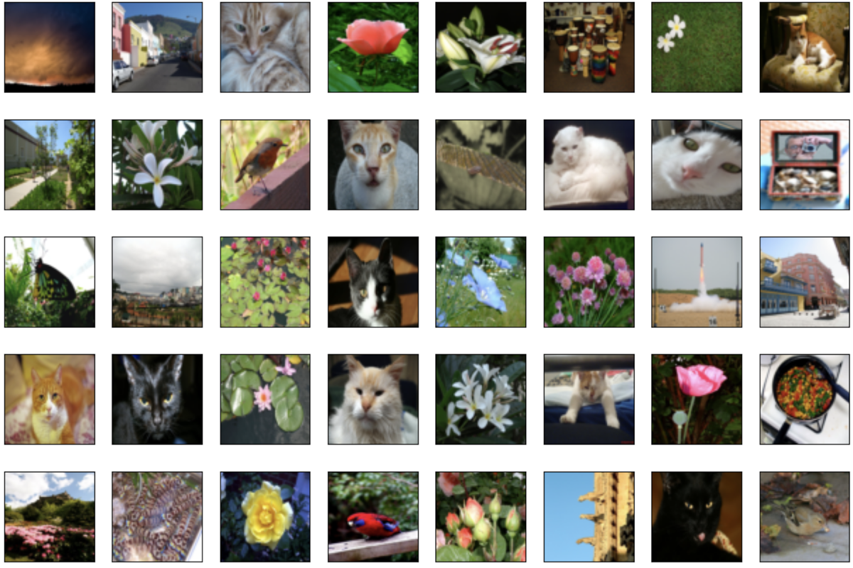
I trained my neural network on a small dataset of over 250 images containing some cat and non-cat pictures.

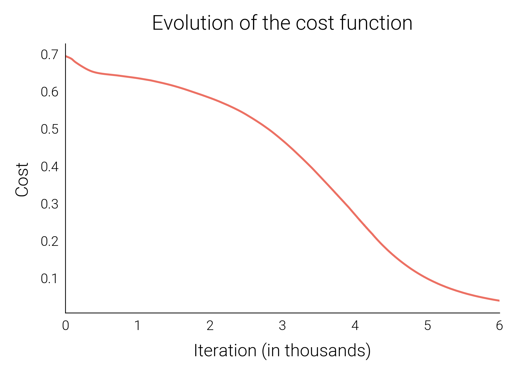
The algorithm worked as expected and so the model was succesfully trained by it. The cost function decreases in each iteration of gradient descent towards a global minimum, as we can see in the plot below.

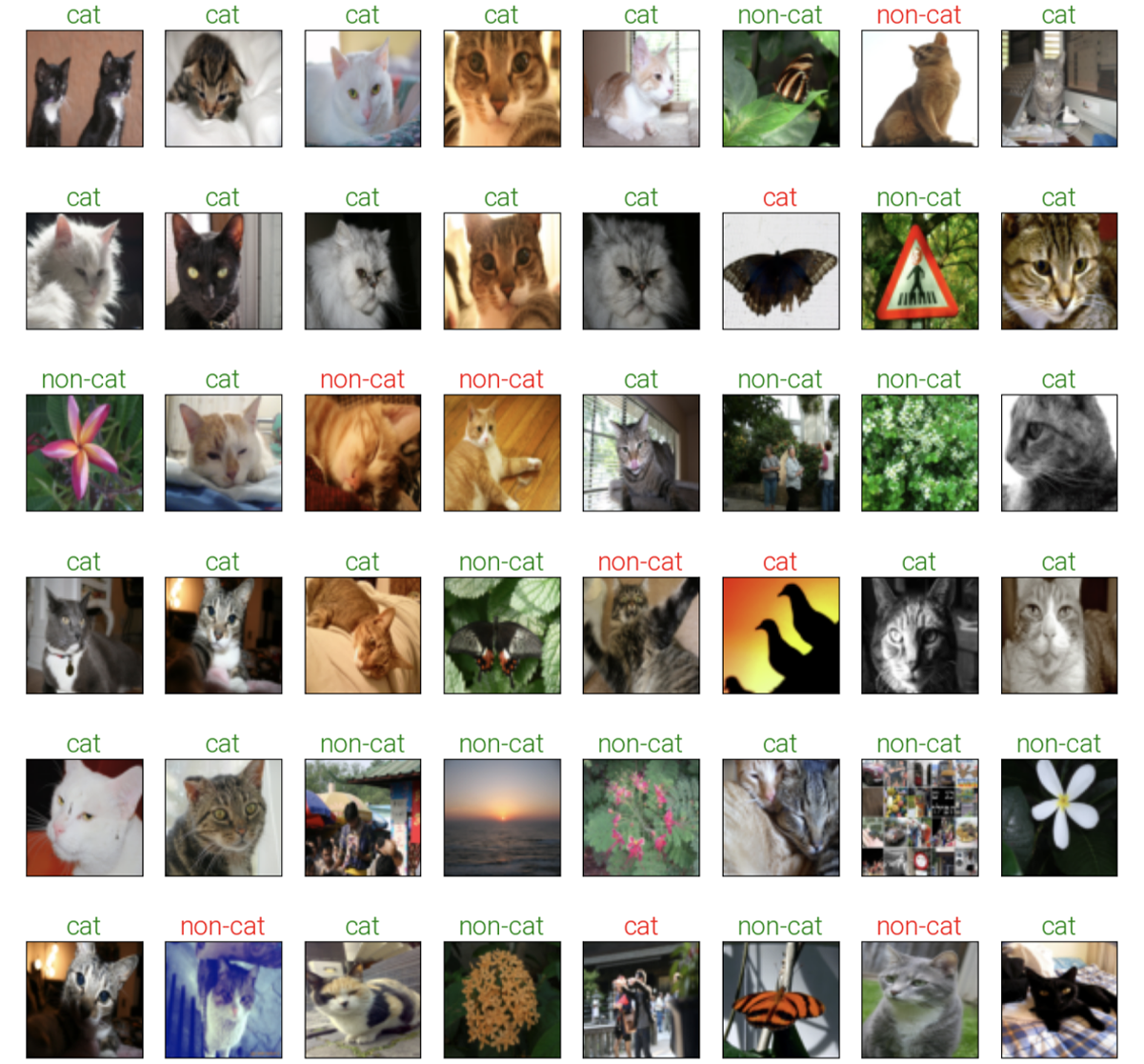
The model was then evaluated on a test dataset, where it achieved an accuracy of 82%. While it’s true that we could potentially improve the performance of the model by utilizing a larger dataset and adjusting the model’s architecture, we’re limited to using only 250 photos for this project. Fortunately, this quantity is sufficient for the project’s objectives. You can see the results here:

4. References
The images used in this project were obtained from the catvnoncat dataset available on Kaggle. This dataset contains 209 images for training, and 50 images for testing, all in color.
5. License
This project is intended for educational purposes only and all materials, including but not limited to code, data, and documentation, are available for free use, modification, and distribution.