Supervised Learning
Personal implementation of logistic regression and linear regression from scratch.

Index:
Introduction
In this side project I am creating from scratch an implementation of linear regression & logistic regression, two pillars of machine learning, with python but without the help of machine learning libraries.
You can check the code here.
Materials
I will be using Numpy’s library to be able to vectorize the computations and make them more efficient. To be able to plot some graphics I will also be using Matplotlib.
Methods
Linear regression and logistic regression consist of finding the optimal parameters \(\vec{w},b\) for our prediction \(f_{\vec{w},b}(\vec{x}^{(i)})\) so that the cost function \(J(\vec{w},b)\) is minimal. Hence, all left to do is solve an optimization problem.
In linear regression, our prediction is \(f_{\vec{w},b}(\vec{x}^{(i)})=\vec{w}\cdot\vec{x}^{(i)}+b\). Associated with this, the most typical cost function used in data analysis is the mean Squared error equal to
\[J(\vec{w},b)=\frac{1}{2m}\sum_{i=1}^m(f_{\vec{w},b}(\vec{x}^{(i)})-y^{(i)})^2\]In logistic regression, our prediction is a bit different since we also have to apply the sigmoid function, \(f_{\vec{w},b}(\vec{x}^{(i)})=(1+\exp(-\vec{w}\cdot\vec{x}^{(i)}-b))^{-1}\), which prevents outliers from messing up the classification. This forces us to change our cost function to make the algorithm efficient (in particular, \(J\) needs to be convex):
\[J (\vec{w},b) = -\frac{1}{m} \sum_{i=1}^m [y^{(i)}\log(f_{\vec{w},b}(\vec{x}^{(i)}))+(1-y^{(i)})\log(1-f_{\vec{w},b}(\vec{x}^{(i)}))]\]This function might look scary, but it’s quite simple. The cost function is the sum of the loss for each sample. And for each sample, the loss function is either the first term (if \(y^{(i)}=1\)) or the second term (if \(y^{(i)}=0\)), and these terms increase as the probabilities worsen. Thus, since the algorithm is minimizing \(J\), we will find the model that computes the best predictions.
In both cases, we will be using Gradient descent: an algorithm that works by driving the parameters \(\vec{w},b\) into the opposite direction of the gradient (i.e. the direction of steepest descent for that point). When computing the gradient (partial derivates), both cost functions result in the same expressions in terms of \(f_{\vec{w},b}(\vec{x}^{(i)})\). Thus the algorithm will update the parameters in each iteration according to the same expression:
\[w \rightarrow w-\alpha \frac{1}{m}\sum_{i=1}^{m}(f_{w,b}(\vec{x}^{(i)})-y^{(i)})x^{(i)}\] \[b \rightarrow b-\alpha\frac{1}{m}\sum_{i=1}^{m}(f_{w,b}(\vec{x}^{(i)})-y^{(i)})\]Since we’re always moving in the gradient direction, we should expect the cost function to decrease in each iteration (given that the learning rate \(\alpha\) is correctly chosen).
Results
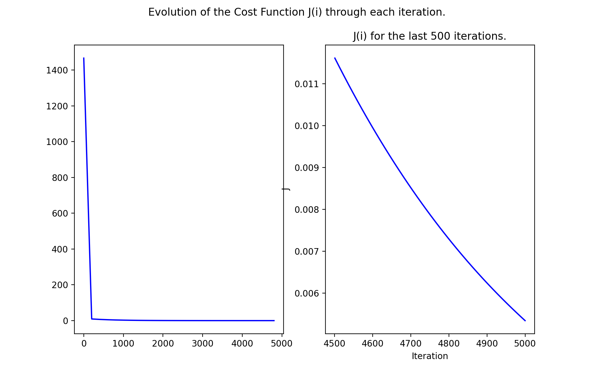
In all test examples, I found that the cost function decreases in every iteration, as expected. All examples followed this pattern:

The optimal parameters found are equal or very close to the ideal parameters for each example:
- Linear regression: Test 1
- The ideal solution is w = 2, b = 10.00
- The solution found is w = 2.01, b = 9.80
- Linear regression: Test 2
- The ideal solution is w = 37, b = -20.00
- The solution found is w = 36.98, b = -19.56
- Linear regression: Test 3
- The ideal solution is w = [5 -5], b = -10.00
- The solution found is w = [5 -5], b = -10.00
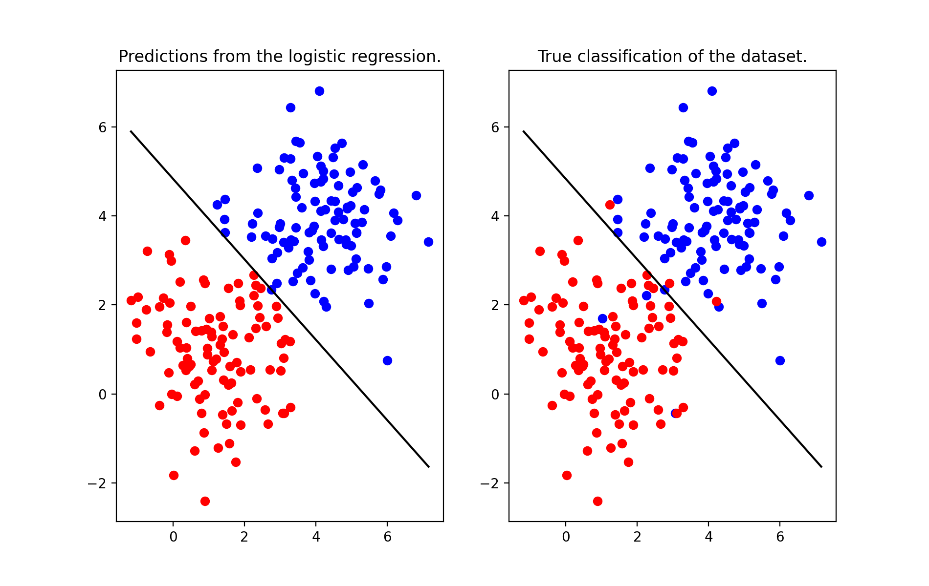
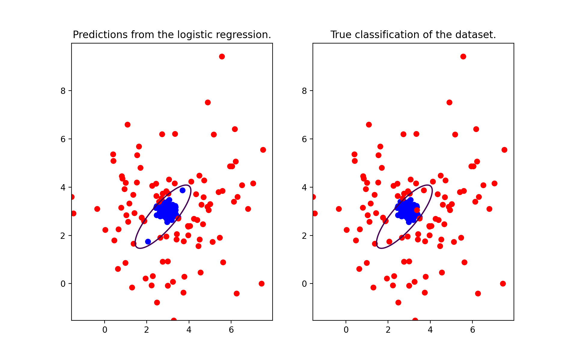
We can visually see that the parameters found for the logistic regression work as well
- Logistic regression: Test 1

- Logistic regression: Test 2

License
This is an educational project; therefore, all materials can be used freely.