Traffic & Air Quality study
Analysis on the relationship between Madrid's traffic flow and its own air quality levels.
Table of Contents:
Introduction
In this project we study the relationship between Madrid’s air quality and the amount of traffic flow through the city center. It’s important to have in mind that the atmosphere is an open system, and thus we expect to find no strong correlation between traffic levels and air quality (since the emissions from vehicles can move to any other area, they don’t have to stay in the city). Basically, we are just checking if there’s a local relationship between traffic flow fluctuations and the levels of concentration of some specific particles. You can check the code here.
Materials and Methods
The methods of this study include the followings:
- Data wrangling
- MySQL
- Data cleaning
- Exploratory data analysis
- ML: Linear regression
- Data visualization (Tableau)
The database consists of more than 100 files, and thus a script was required to automate the process for a fast data merge. Because of the nature of our study, we also had to aggregate our data by weeks.
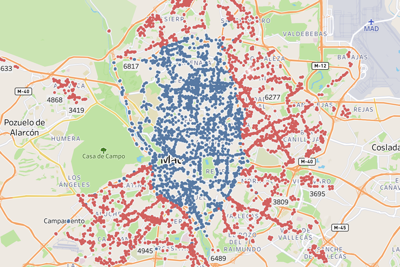
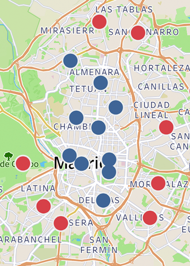
The study only focuses on the city center, and thus some stations had to be filtered out, as we can see below.
We have data for the traffic flow. However, we do not have data on the individual flow \(j_i\) of each category of vehicle (cars, motorbikes, buses, etc). We suppose the individual flow is just dependant on the proportion of circulating vehicles of that category, \(j_i = J \times n_i/n_T\). However, we do not know \(n_i\) (number of circulating vehicles of category i) nor \(n_T\) (total number of vehicles circulating). So we approximate this value: we make the assumption that the proportion of accidents of vehicles i (\(acc_i/acc_T\)) is proportional to the proportion of vehicles i circulating, that is \(n_i/n_T \approx \alpha_i \times acc_i / acc_T\). And so we have:
Since we have data for \(n_i/n_T\) for two specific years: 2017 and 2013, we can use both to compute the constant of each category in each year, and then choose our coefficients as the mean of both. We will then use it for the rest of the years.
Finally, we model their depedency through a linear regression in order to understand the impact of traffic in the local Air Quality (we see this in the next plot).
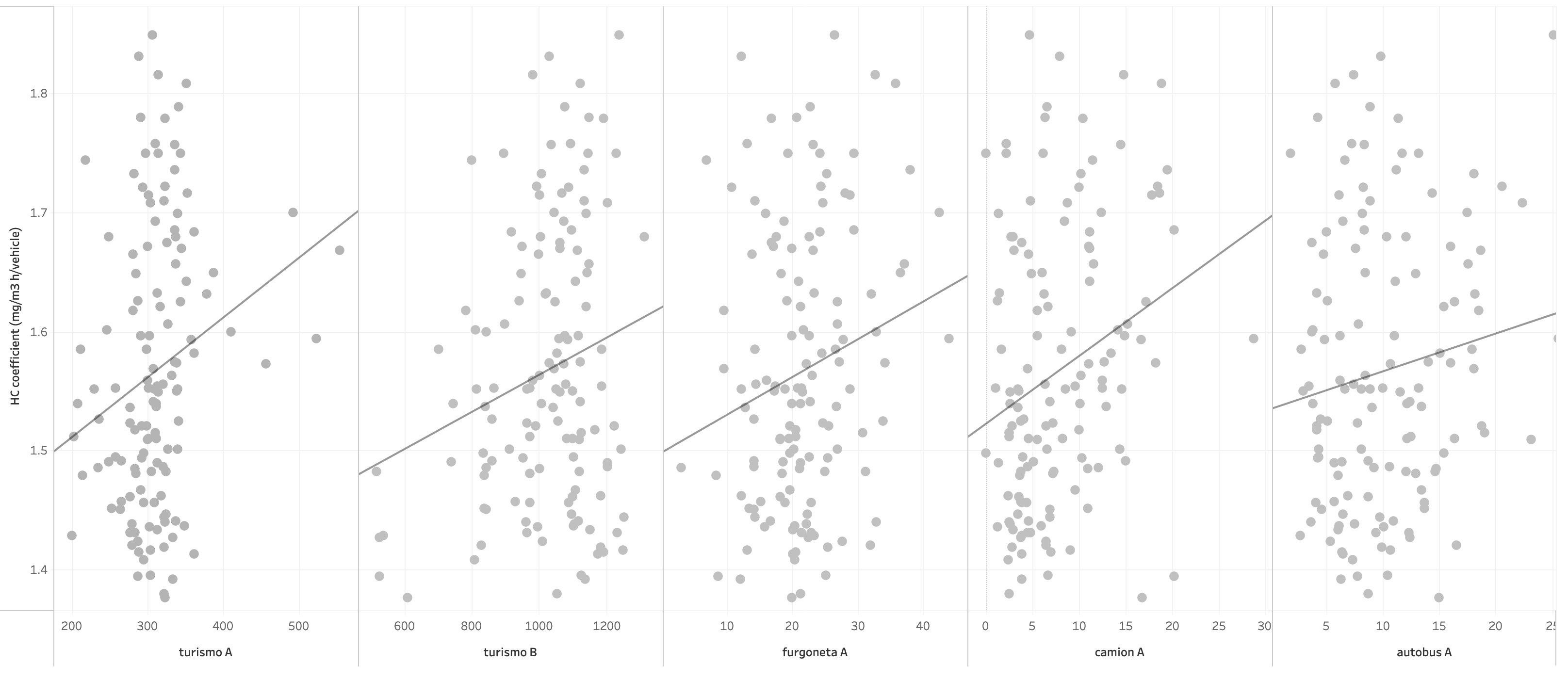
From this graph we can see how each vehicle flow affects the local air. However, the scales are not the same. Hence, we create a new bar plot to compare the value of the slopes with impartiality.
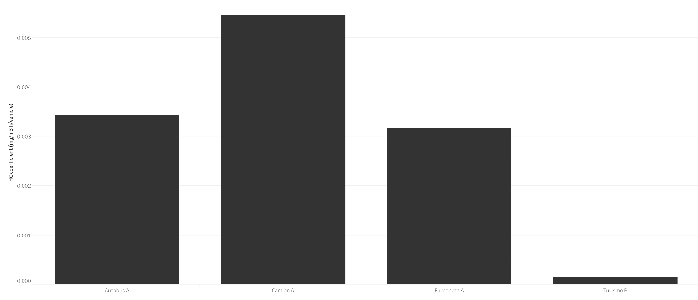
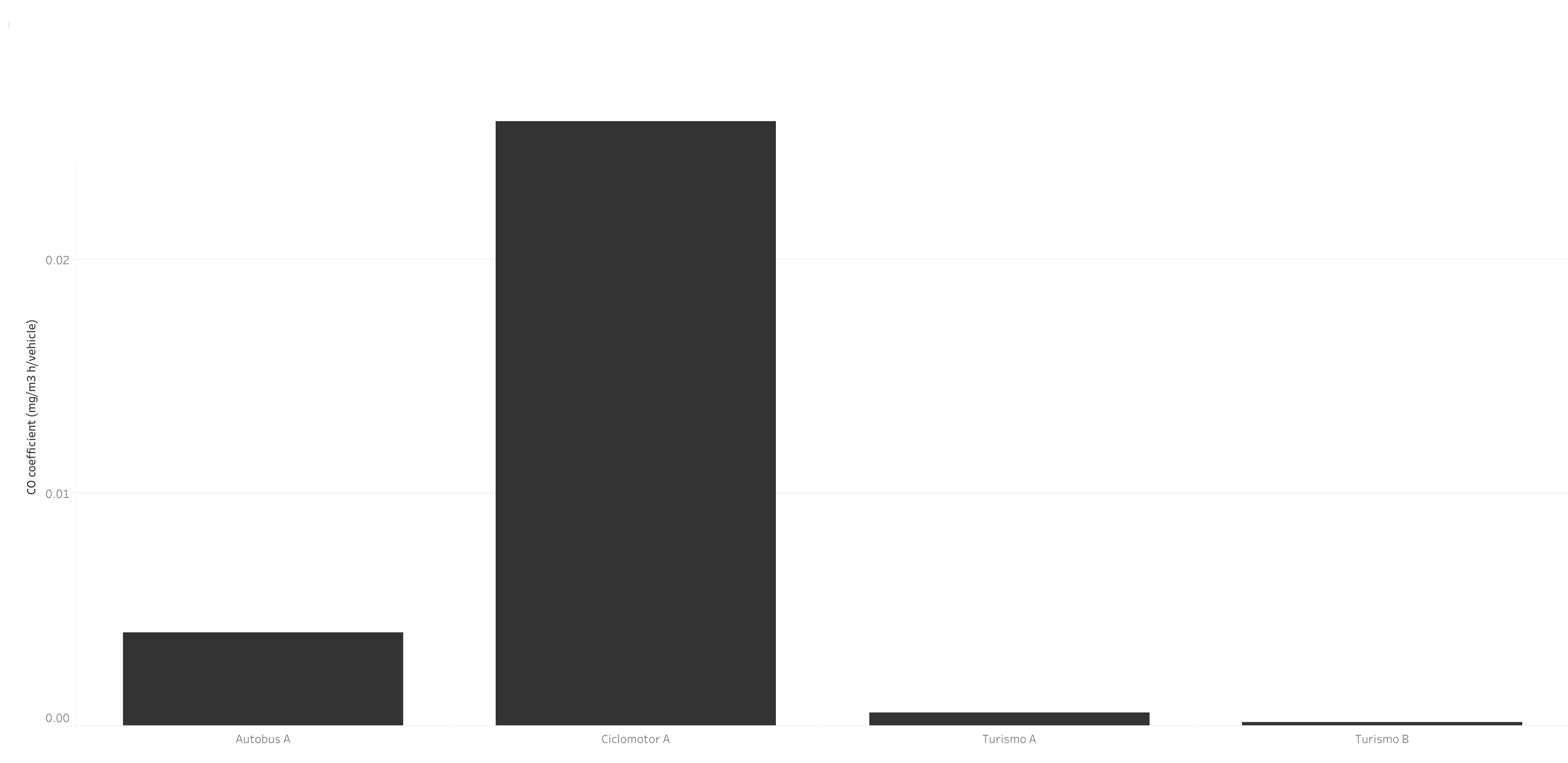
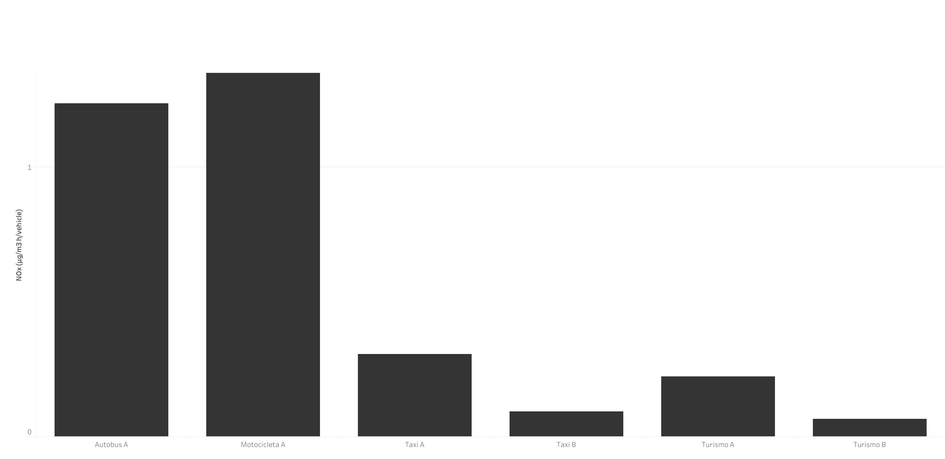
These values represent the amount of local emissions an individual vehicle is related to. It’s important to understand this: the slopes represent how pollution would rise if we were to increase the number of vehicles of type \(i\) (it’s not the total pollution from each vehicle type).
Results
Carbon monoxide (CO)
Scouters are allowed to emit higher concentrations of CO, and thus we did expect these results.
Hydrocarbon (HC)
Heavy vehicles such as Buses, Trucks and Vans were the most related to local HC emissions in our data.

Nitrogen oxides (NOx)
According to our data, motorbikes and buses were the most polluting towards local NOx.
References
The air quality and traffic flow data was sourced from Madrid’s Data Portal. This portal provides open access to a wide range of data and information on the city of Madrid, including environmental and transportation data. All data used in this report was obtained from the Madrid Data Portal and is subject to their terms and conditions of use.
License
This is an educational project; therefore, all materials can be used freelly.